

____
Having found the underlying algorithms based on fundamental laws of fluid mechanics and acoustics which enable the calculation of sound levels of compressible fluids emanating from control valves, and thereby simplifying the IEC Standard and improving accuracy, I thought that a similar method applying to gases might also be good. However this task proved to be quite difficult. After much time and effort I finely was able to compress over 40 equations of an IEC prediction standard into three graphs plus a few modifiers. I thought such a simplified graphical method might be a handy alternative to a computerized method. While this method,as exhibited, is valid for air, it could be modified for other gases as long as the specific gravity and sonic velocity are accounted for (see adjustments below).

Graph A. This graph encompasses
the relative valve flow coefficient,
and the downstream pipe size
1) The first graph A shows sound levels as function of the given valve’s outlet pipe diameter(D) either in inches or in mm, and as function of the relative flow capacity (Cv / D2);D in inches, or Cv /(0.04 x d)2 if d is given in mm. The graph also incorporates the pipe’s transmission loss based on schedule 40 pipe (for schedule 80 see below). Note: Cv is based on actual process conditions.
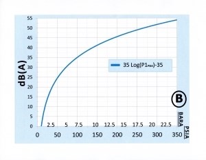
Graph B. Relates to the inlet pressure of the valve
2) The next step is to consult Graph B based on the absolute inlet pressure to the valve either in psia or in bar absolute. Find the appropriate dB(A) numbers corresponding to the valve inlet pressure and add it to the results from Graph A. Then proceed to Graph C.
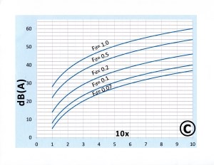
Graph C. Is based on the actual pressure drop
across valve modified by the Fd factor of
the given valve.
3) In Graph C, the first step is to find the valve’s pressure ratio, where X = (P1 – P2 / P1), here P1 is the absolute inlet pressure and P2 the absolute outlet pressure. Multiply X by ten and find the corresponding 10X number on the bottom of the graph. Read up to the curve agreeing with the Fd numbers of your valve. Fd affects the diameter of the noise producing jet. Next read the corresponding dB(A) number on the left. (Use the “Tabulation of Fd – Factors” below for estimating purposes in case you don’t know your valve’s Fd number).
| Tabulation of Fd – Factors | ||||||||||
| CV/D2 (D in inches) | 3 | 6 | 9 | 12 | 15 | 18 | 21 | 24 | 27 | 30 |
| (Cv/d2) x 103 (mm) | 4.64 | 9.3 | 14 | 18.6 | 23.3 | 28 | 32.6 | 37.2 | 42 | 54 |
| Globe valve, parb. plug* | 0.27 | 0.31 | 0.39 | 0.46 | ||||||
| Butterfly valve | 0.45 | 0.30 | 0.33 | 0.40 | 0.45 | 0.48 | 0.50 | 0.53 | 0.55 | 0.57 |
| Segment. ball valve | 0.60 | 0.62 | 0.65 | 0.68 | 0.72 | 0.73 | 0.75 | 0.77 | 0.78 | 0.80 |
| *Flow to open |
- If your pipe is schedule 80, add 4 db(A).
- If this is a rotary valve, add rw = 3 dB to the total.
- A = 7.3 dB(A) for 2” (50 mm) size and a Cv/D2 of 3.1 or, 12.5/(0.04 x 50)2 = 3.1 also for d in mm.
- B = 30.1 dB(A) for P1 of 72.5 psia (5 bara)
- C = 34 dB(A) based on 10X = 8 = 10x (P1–P2/P1) and Fd = 0.07

Fig. 1. Shows actual flow rest results on a 2” (DN 50)
valve installed in a 2” pipe. The medium is helium.
The comparative results indicate the proposed
method seemed to work well even though
the gas in the downstream pipe reached
subsonic velocities.
Note: This method is not applicable when a valve is installed in an enlarged outlet pipe when the valve’s outlet velocity into the expander exceeds 0.3 Mach. Valves without expanders are exempted from this rule (see Figure 1).
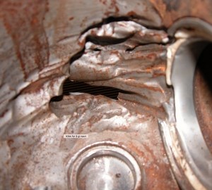
Fig. 2. Here, test data is based on air using a
8” segmented ball valve having a 400 mm (16”)
downstream pipe. Here the predicted sound level
matches reasonably well except at high pressure
ratios. The reason is, that at X = 0.7 (7 = 10X)
the pipe outlet velocity exceeds 0.2 Mach,
indicating the proposed method accepts high
outlet velocities only when the pipe size
matches that of the valve.
- Inlet pressure 2.8 dB
- Density of gas 0.4 dB
- Pressure drop 1.4 dB
- FL factor 1 dB
- Fd factor0.8 dB
- Flow coefficient (Cv/Kv) 0.4 dB.
- Baumann, Hans D. A simple aerodynamic noise estimating method: Why not? VALVE WORLD, November 2016, pp 111-116.
- IEC Standard 60534-8-3 Control valve aerodynamic noise prediction method. International Electrotechnical Commission, Geneva, Switzerland.