Cavitation risk assessment using CFD simulations

Traditionally, cavitation assessments rely on time-consuming flow loop tests or complex multiphase CFD simulations. This article presents a more efficient alternative: using single-phase CFD simulations with pressure field correction to calculate key cavitation risk indicators like the incipient cavitation index σ_I and liquid pressure recovery factor F_L.

By Praveen Kumar Ramachandran, Centre for Computational Technologies

The hidden cost of cavitation

Cavitation in control valves can lead to noise, vibration, reduced performance, material damage, and shortened service life. It occurs when pressure drops below the vapour pressure, forming vapour bubbles that collapse downstream, generating destructive microjets and shock waves. These forces can severely damage the valve surface, causing pitting and erosion. Cavitation risk is particularly high in control valves operating under severe service conditions, characterised by high pressure drops.

Methods to combat cavitation

Strategies to address cavitation include:

• Avoid cavitation: Elevating operating pressure to maintain flow pressure above vapour pressure.
• Robustness: Using high-strength materials to withstand erosive forces.
• Isolate cavitation: Directing collapsing bubbles toward the centre of the flow, to minimise surface damage.
• Eliminating cavitation: Designing the valve to drop the pressure in stages using an
  anti-cavitation cage or inserts, to prevent the formation of vapour bubbles.

The last two methods require careful valve flow path design, with staging the pressure drop involving gradual pressure reduction through the valve trim. These approaches often require multiple design iterations to optimise pressure conditions. Specific parameters are needed to assess cavitation intensity, allowing designers to evaluate and compare design solutions for the most effective outcome.

Parameters to assess cavitation

To assess the cavitation risk in control valves, two key parameters are commonly used: the Cavitation Index (σ) and the Liquid Pressure Recovery Factor (F_L). Cavitation Index (σ) – Three terms are commonly used to classify cavitation in valves according to the International Society of Automation (ISA-RP75.23-1995):

1. Incipient cavitation: The start of steady cavitation, indicated by an intermittent popping sound in the flow stream.
2. Constant cavitation: Indicated by a continuous popping similar to the sound of gravel flowing through the pipe
3. Choking cavitation: Occurs when the valve is passing the maximum flow possible for a given upstream pressure

The cavitation index is typically used to predict cavitation level and is calculated as follows
(International Society of Automation, ISA-RP75.23-1995):

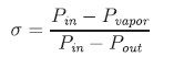
The operating cavitation index can be compared against the published cavitation indices (incipient, constant, or choking) to predict the level of cavitation. A valve’s cavitation indices for incipient, constant, and choked levels can be determined from flow loop tests conducted in accordance with ANSI/ISA 75.02.01. Cavitation can be observed using a hydrophone or accelerometer during the test. A graph of the logarithmic accelerometer output versus flow rate or cavitation index is plotted. The slope of this curve normally changes at the points of incipient, constant, and choking cavitation, as shown in the image. The lower the calculated operating cavitation index value is, the greater the likelihood of cavitation damage.

Liquid pressure recovery factor F_L

F_L is the liquid pressure recovery factor of the valve. This factor accounts for the influence, of the valve internal geometry on the valve capacity at choked flow. The formula for the Liquid Pressure Recovery Factor is:

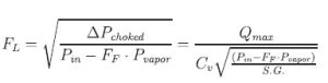
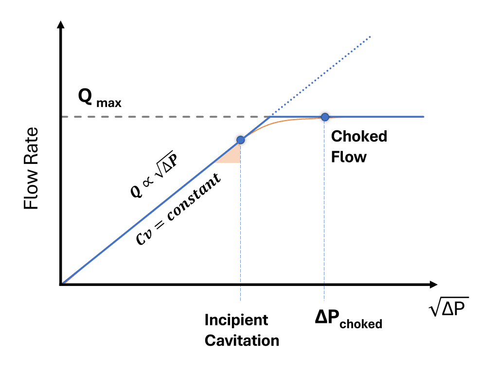
The maximum flow rate, Q_max, is required in the calculation of the liquid pressure recovery factor, F_L. For a given upstream pressure, the quantity Q_max is defined as that flow rate at which a decrease in downstream pressure will not result in an increase in the flow rate (horizontal line in image). The test procedure to calculate F_L is described in ANSI/ISA-75.02.01. Designers can use these parameters to optimize flow paths and make informed design decisions.

Computational Fluid Dynamics (CFD)

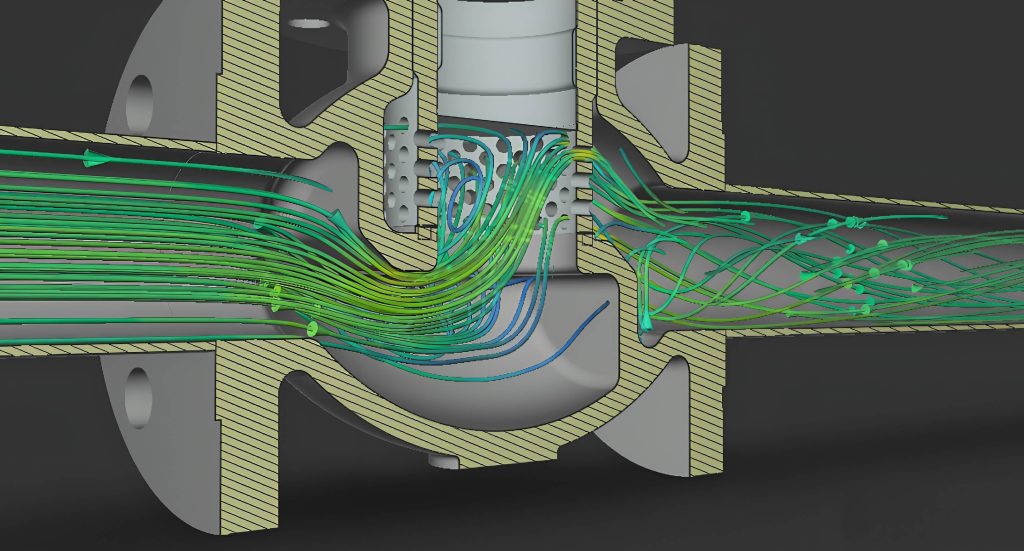
Computational Fluid Dynamics (CFD) simulation uses numerical methods to solve fluid flow, heat transfer, and related phenomena. The fluid domain is divided into discrete mesh cells and the governing Navier-Stokes equations are solved in each cell. The Reynolds-Averaged Navier-Stokes (RANS) approach is typically used to model the turbulent behaviour of flow.

Validation study: sharp-edge orifice

This validation study compares CFD results with experimental data from “Calibration and Verification of Cavitation Testing Facilities Using an Orifice” by William Rahmeyer and Fred Cain. The orifice, with a 1.534-inch throat diameter, was tested across seven laboratories. For this CFD validation, data from Lab B was selected. The orifice was modelled as 2D axisymmetric geometry, with the fluid domain meshed using quadrilateral cells and prism layers near the orifice edges for accurate flow resolution.

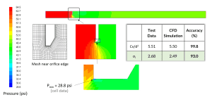
Step 1: Single-phase flow simulation for incipient cavitation index

The first step is the single-phase flow simulation to determine the flow capacity C_v and the incipient cavitation index. The inlet pressure was set to 50 psig (64.7 psi absolute), and the outlet to 50 psi absolute, resulting in a 14.7 psi (1 atm) pressure drop. The simulation showed a minimum pressure of 28.8 psi, which was used to calculate the σ_I. The CFD results closely matched the experimental data, confirming the simulation’s accuracy.

Step 2: Multi-phase flow simulations for liquid pressure recovery factor

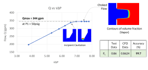
The next step is multi-phase flow simulations to determine the maximum flow rate at choked flow (Q_max) in order to calculate the F_L. The mixture multiphase model was used to capture the liquid and vapour phase in cavitating regime. A series of simulations were conducted by reducing the outlet pressure while maintaining a constant inlet pressure. In the non-cavitating region, the C_v remained constant – the flow rate was proportional to the square root of pressure drop. However, as the pressure drop is increased by reducing the outlet pressure, the flow crossed the incipient cavitation threshold, transitioned into the cavitating region, and reached the choked condition where the flow rate doesn’t increase any further. The Q_max obtained at choked flow was then used to calculate the FL. The CFD results closely matched the experimental data, confirming the accuracy of the simulations.

Challenges in CFD simulation

CFD simulations present several challenges, including:

• High mesh refinement: Required for accurate flow resolution. High mesh count increases computational cost, especially for complex control valve geometries.
• Multiphase simulations: These are computationally heavy, requiring multiple iterations to reach choked flow and repeated for each valve opening to generate a full FL plot.
• Slow Convergence: The pressure inlet – pressure outlet boundary conditions can be unstable, resulting in slow convergence.
• High computational time and cost: Due to the complexity of multiphase flow simulations, the overall computation time and cost are significantly high.

Proposed alternate method: pressure field correction

The proposed method leverages single-phase flow simulation results to determine F_L In an incompressible flow simulation, the computed pressure field allows for adding or subtracting the same pressure value across all cells without affecting other flow variables. Hence, the pressure field obtained from single phase flow simulation (step-1) is adjusted to mimic a choked flow by subtracting a constant value, without any additional simulations. During this process, the pressure contours are visualized, with a color scale that distinguishes areas where the pressure is greater than the vapor pressure (blue) from areas where it falls below the vapor pressure (red). The pressure field is iteratively corrected until the contour plot shows a complete blockage of the flow path, with the red region. This condition is considered to approximate choked flow. From this corrected pressure field, the liquid pressure recovery factor FL can be calculated using the upstream pressure, pressure drop, and vapor pressure values. When applied to the sharp-edge orifice validation case, the proposed method produced excellent agreement with the lab data as well as the results from conventional CFD simulations.

Case study: 1.5” full port ball valve

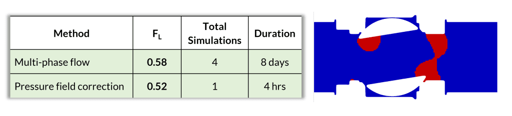
In this case study, a 1.5-inch full port ball valve was evaluated at 80° opening. The liquid pressure recovery factor (F_L) was calculated using both the conventional multiphase flow approach and the proposed pressure field correction method. The results from both approaches were within 10% difference.

Case study: 8” double offset butterfly valve

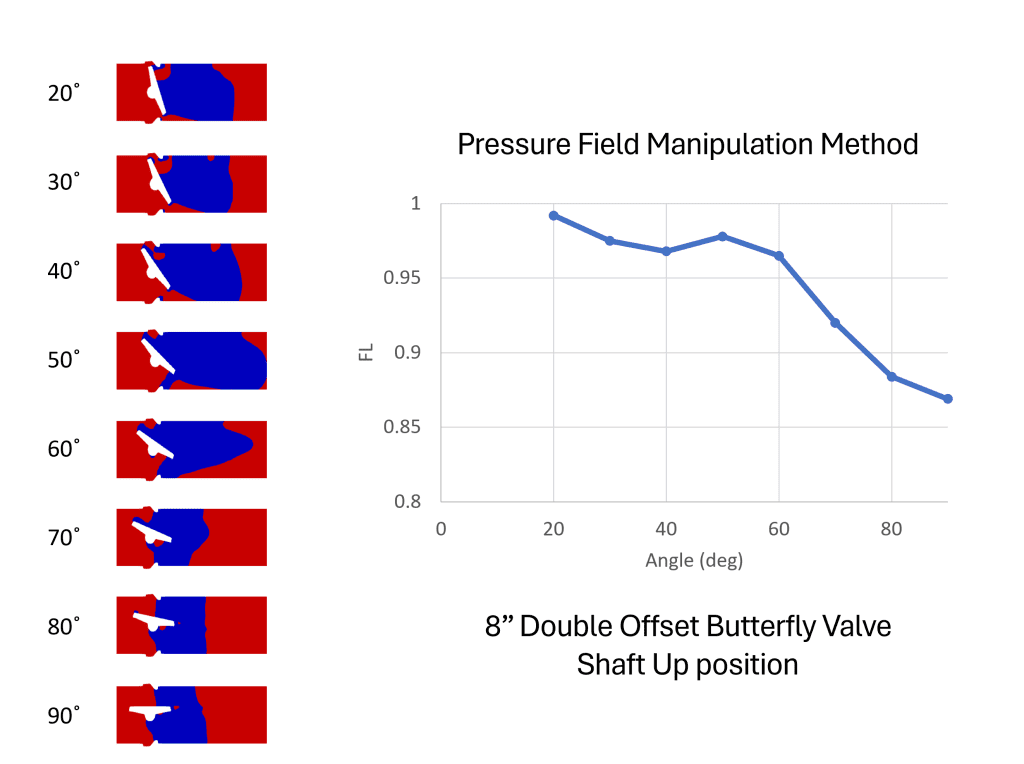
In this case study of an 8” double offset butterfly valve, the pressure field correction approach was used to calculate the FL for each valve opening from 20° to 90°. The resulting FL values are presented below. The FL vs. valve opening plot shows the typical pattern observed for a double offset butterfly valve,  demonstrating the method’s effectiveness in capturing expected performance trends

Summary

The proposed pressure field correction method offers significant advantages in time efficiency, enabling quick estimation of FL with accuracy within 10% of conventional multiphase methods. This approach allows for fast design iteration comparisons, making it ideal for valve design optimization. However, detailed multiphase flow simulations are required for the final design to obtain accurate results. A key limitation of the proposed method is that the contours obtained do not accurately represent actual choked flow. While the FL values are quickly predicted, the method may not capture all complexities of cavitation. Despite its promising results in the orifice and other case studies presented, the method requires further validation across various valve types.

About this Technical Story

This Technical Story is an article from our Valve World Magazine, August 2025 issue. To read other featured stories and many more articles, subscribe to our print magazine. Available in both print and digital formats. DIGITAL MAGAZINE SUBSCRIPTIONS ARE NOW FREE.

“Every week we share a new Technical Story with our Valve World community. Join us and let’s share your Featured Story on Valve World online and in print.”