
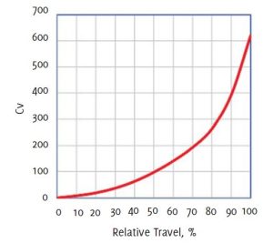
Q. I need to specify a control valve for a liquid system involving very short runs of pipe both upstream and downstream of the valve. The source pressure will remain constant at all specified flow rates. The back pressure from the receiving equipment will also remain constant at all specified flow rates. Normally I would specify a globe control valve with a linear inherent flow characteristic. The problem in this case is that the fiber content of the process media is too high for a globe valve. In similar processes in my plant, but with longer pipe runs, we satisfactorily use segment ball valves, which are only available with an equal percentage inherent flow characteristic. I have attached a Cv vs. relative valve travel graph for my preferred manufacturer’s segment ball valve. (Figure 1.) Can you suggest a solution for this application?
A. What I have done in similar situations is to add a flow modification block in the output of the controller, something that is usually easy to do with modern digital controllers. The first step is to normalize the vertical scale on the manufacturer’s Cv chart so that instead of reading in units of Cv it reads in relative Cv, that is from zero to 100 percent of the fully open Cv (Figure 2, A).
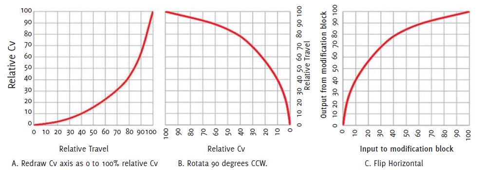
Then rotate your relative Cv vs. relative valve travel graph 90 degrees counterclockwise (Figure 2, B). Finally, flip the graph horizontally (Figure 2, C). You now have a modification graph to enter into your controller’s modification block. Although the text and numbers look a bit strange, upon relabeling the horizontal and vertical axes, as shown in Figure 2, C you have a graph in a conventional format that you can use to program your modification block.
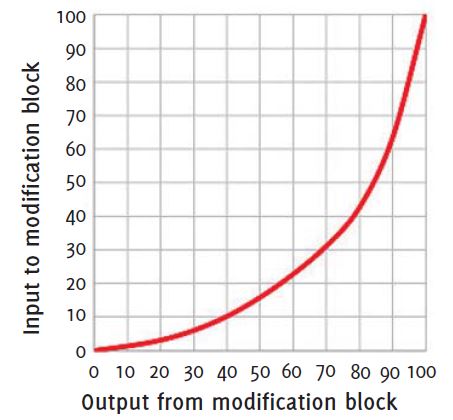
Once you are satisfied that creating the modification block graph is based on a logical sequence, you can save a lot of time by simply relabeling the Figure 2, A graph as shown in Figure 3. Granted, it is not in conventional form (input, horizontal axis, output vertical axis), but no one will see it except you.
flow range, making it more difficult to come up with a set of controller tuning parameters that will result in fast and stable control. One well-known valve manufacturer (Neles) includes installed flow graphs in its valve sizing application, and at least one other can furnish installed flow graphs on request. There are also three sets of Excel worksheets on my website that graph control valve installed flow. The simplest of them is listed on the website as “Control valve sizing worksheets.”
The download consists of three Excel worksheets, one for liquid, one for gas flow in volumetric units, and one for gas flow in mass flow units. On the Installed flow tab of each is a space to enter a table of Cv and of xT or FL of the valve you want to analyze. There is a more comprehensive set of sheets listed on the website as “Control Valve Sizing application workbooks”.
These Excel Workbooks are intended as full function control valve sizing applications and have built-in Cv tables for a variety of generic control valve styles. The worksheets in both these sets include valve noise prediction calculations in accordance with the current IEC control valve noise prediction standards.
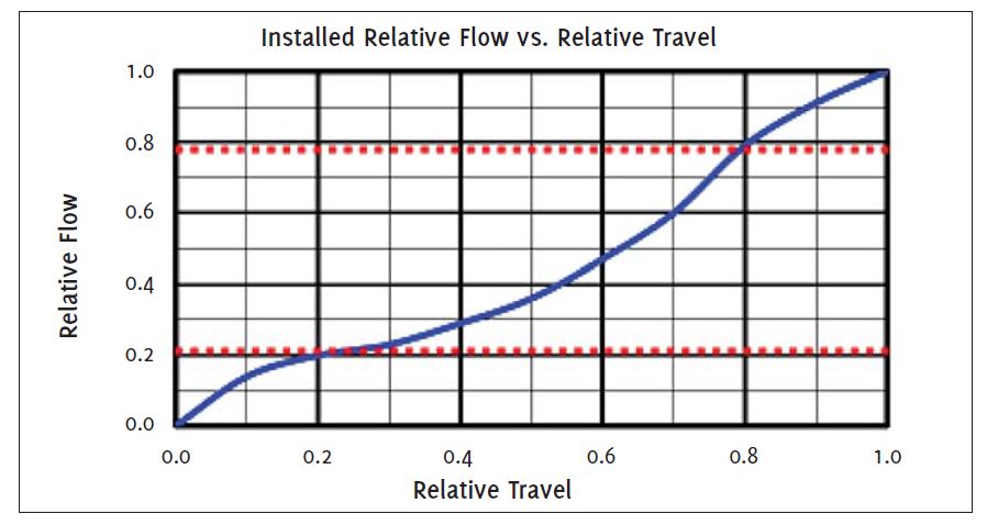
The most popular worksheet, which is labelled “Enhanced version of graphing control valve installed flow and gain”, makes it possible to create installed flow graphs in conjunction with the user’s preferred control valve application. Figure 4 is an installed flow graph made using this Excel sheet. The installed flow characteristic is pretty good as is, but since it is so easy to do, it could be helped a bit by applying the same method used in linearizing an equal percentage inherent flow characteristic.
About the author
Jon F. Monsen, PhD, PE, was a control specialist with over 45 years of experience in the control valve industry. He lectured nationally and internationally on the subjects of control valve application and sizing. Jon’s website, www.Control-Valve-Application-Tools.com freely shares articles, training and professional development materials, and Excel worksheets that might be of interest to those who use or specify control valves. Jon passed away in December 2023 and his series of columns is being published in accordance with his wishes.
About this Technical Story
This Technical Story is an article from our Valve World Magazine, March 2024 issue. To read other featured stories and many more articles, subscribe to our print magazine. Available in both print and digital formats. DIGITAL MAGAZINE SUBSCRIPTIONS ARE NOW FREE.
“Every week we share a new Technical Story with our Valve World community. Join us and let’s share your Featured Story on Valve World online and in print.”