
This article introduces a streamlined approach to predicting hydrodynamic sound levels in throttling valves, which requires solving only 6 equations compared to the 22 equations of the IEC standard method, making it more accessible while maintaining reasonable accuracy.
By Hans D. Baumann
While cavitation annoys us with unpleasant noise, one must not forget the economic impact it has. There is a direct correlation between valve damage and sound level. A typical reference is that cavitation damage starts when sound levels exceed 80 dBA.
Mind you, any liquid, even our own blood, can cavitate. In the 1960s, people used double-seated globe valves to control flow in crude oil pipelines. One part of a double-seated parabolic plug saw a flow direction “to close”. As a result, this part saw high pressure recovery, hence low FL and low Xfz factors. Such valves suffered much cavitation damage and eventually got replaced by ball valves.
The mechanism of cavitation and sound creation
Most of us know that when throttling liquids reaches a static pressure at the vapor pressure, parts of the liquid create little vapor gas bubbles. These later implode when the velocity is reduced with a corresponding higher static pressure, causing the vapor bubbles to implode. Those implosions create sonic velocities which in turn create an erosive impact on metal and corresponding sound waves. This happens when the rest of the liquid still undergoes turbulence. The result is that the overall sound we perceive is the combination of turbulence plus cavitation sound.
To understand the sound creation mechanism, one must realize the sound we hear is actually the frequency of the turbulent liquid. The frequency of the imploding gas bubbles happens above 10,000 Hertz, hence in the inaudible range.
Turbulent sound is created if liquid velocity (Uvc) reaches 103 ft/s while cavitation sound follows Uvc6 if the ratio = (P1-P2) / (P1-Pv) exceed Xfz; there are other factors affecting sound, such as the pipe size, the pipe’s wall thickness and the valve’s flow capacity (Cv) (see my equation factor A below).
Finally, there is the inlet pressure (B) in my equations which affects sound at the 3.5th power. Hence, 35 log (10 P1)-35.
Simplified sound prediction method
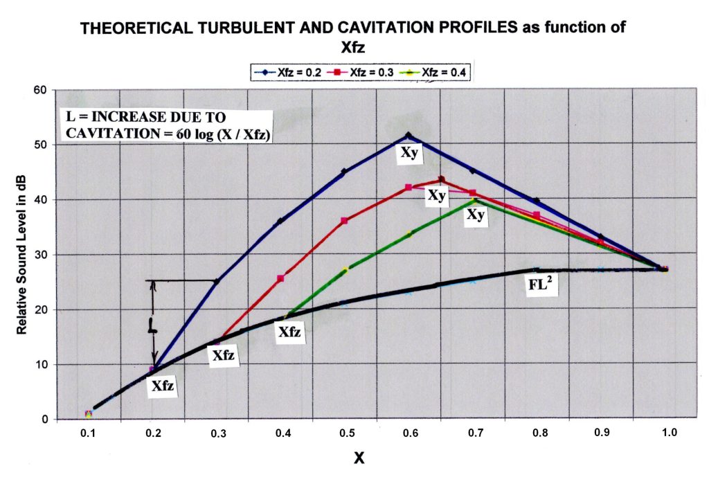
To understand how this all goes together and to understand my simplified sound prediction method, I propose to create a test diagram plotting sound level in dBA against X. Since there is no sound at X = 0, we need to start with a basic foundation, namely A + B. Assuming A+B = 58.5 dBA, this is the starting point in the graph. Now we calculate the sound level at X = 1, which, for turbulence, is 30log(1×10) = 30 dBA. Connecting 58.5 at X = 0.1 to 30 + 58.5 at X = 1 by a straight line, we have the predicted sound level for any X values up to X = FL2. Why FL2? Because at this pressure ratio, the liquid gets choked and there is no more flow increase.
Similar graphs can be made to connect Xfz to Xy at a rate of 60 log (X / Xfz) to predict cavitation, and a final line between Xy and the turbulent sound line using a slope of 120 log (X / Xy) to predict decreasing cavitation sound. See Figure 1 below.
Estimating sound levels for actual throttling valves
Having explained the basics, let’s try to estimate sound levels for actual throttling valves. The sound level in dBA is the summation of several equation blocks plus modifiers.
SPLAe = A + B + C + rw + modifier A = 8 log (D) + 12 log(Cv/D2) + 4. Here, D is the nominal pipe diameter in inches, Cv is the flow capacity of the pipe (at the valve’s outlet) in gallons per minute (a proxy for kg/sec mass flow).
B = the valve’s inlet pressure in psia3·5, or 35 log(P1) – 35.
C = c1 + c2 + c3, where c1 defines turbulence, c2 defines cavitation and c3 defines decreasing cavitation.
C1 = 30 log(10X), c2 = 60 log (X / Xfz), note that X max. = FL2. c3 = -120 log (X / Xy).
Xfz = coefficient of incipient cavitation (valve specific), ranges between 0.2 to 0.5. As an estimate, use FL0·5. Xy is X at max cavitation and destructive power. Xy = (Xfz + 1) / 2. rw = -3 (for globe valves only).
An example
An example may be helpful. Consider a 4-inch V-port valve with Cv = 93.5, P1 = 145 psia, Fl = 9.9 and Xfz = 0.35. X = 0.5,
Xy = 0.68, rw = -3.
A = 8 log (4) + 12 log (93.5 / 42) + 4 = 3.5 + 9.2 + 4 = 16.7 dBA. B = 35 log(145) – 35 = 40.6 dBA. A + B = 57.3 dBA. This would be the sound level at X = 0.1.
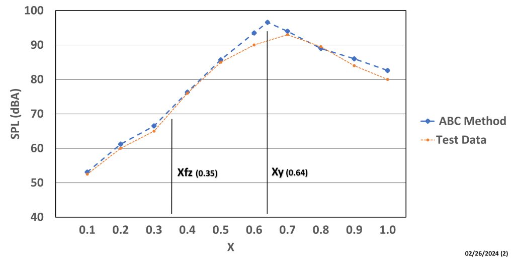
C1 = 30 log (10 x 0.5) = 21 dBA. c2 = 60 log (0.5 / 0.35) = 9.3 dBA. c3 = -120 log (0.5 / 0.68) = 0 dBA (since no positive value). This makes C = 21 + 9.3 + 0 = 30.3 dBA.
The total sound level at X = 0.5 now is A + B + C + rw = 16.7 + 40.6 + 30.3 – 3 = 84.6 dBA. This compares to 85dBA in the test data shown in Figure 2.
Other prediction methods
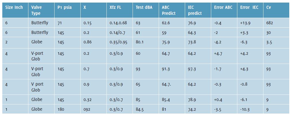
One of the pioneers of a reasonable hydrodynamic sound prediction method was Kiesbauer¹. His method was based on equations from curve fitting of test data. This works well for certain test valves but could not be applied to other types of valves. Then came the IEC Standard 60-534-8-4 on hydrodynamic sound prediction² for control valves. While it is reasonably accurate (see Table 1), it is not widely used, in part due to a need to solve 22 equations (compared to only 6 equations for the ABC method). It is based primarily on empirical equations and requires certain vendor-based, valve-specific coefficients, which are unavailable to the general public. A recent publication is by Baumann³.
References
- Kiesbauer, J. 1998. “An improved prediction method for hydro-dynamic noise in control valves.” Valve World Magazine, 3(3), pp. 33-49.
- IEC Standard 60534-8-3, 2005. “Prediction of noise caused by hydrodynamic flow.”
- Baumann, H. D., 2024. “Sound pressure slopes of turbulent and cavitating liquids, and methods to predict such Levels.” ASME Open Journal, Vol. 3, 031008-1.
About the author
Dr. Hans D. Baumann is an internationally renowned consultant with extensive experience in the valve industry. Throughout his career, he held managerial positions in Germany and France, and his innovative spirit led to the creation of 10 novel valve types, including the well-known Camflex valve. Dr. Baumann has authored 8 books, including the acclaimed “Valve Primer,” and has been granted 115 US patents. He also founded his own valve company, which he later sold to Emerson, and served as Vice President at Masoneilan and Fisher Controls Companies. The author can be reached at: hdbaumann@phbinc.net
About this Technical Story
This Technical Story is an article from our Valve World Magazine, August 2024 issue. To read other featured stories and many more articles, subscribe to our print magazine. Available in both print and digital formats. DIGITAL MAGAZINE SUBSCRIPTIONS ARE NOW FREE.
“Every week we share a new Technical Story with our Valve World community. Join us and let’s share your Technical Story on Valve World online and in print.”